Predicting the Distribution of Tree Species and Their Biomass in Yangambi Biosphere Using Spatial Interpolation

Received 14 Jan, 2023

Accepted 06 Jun, 2023

Published 30 Sep, 2023

Background and Objective: Knowledge of the spatial distribution of trees and stands is very important in forest management strategies. This study investigated whether spatial interpolation methods could predict the spatial distribution of tree species and their biomass in a mixed forest of Yangambi Biosphere, Democratic Republic of Congo. Materials and Methods: A 90×90 m grid was installed in a mixed forest, the coordinates of each selected tree were recorded with a GPS and the Diameter at Breast Height (DBH) measured. The 3 biomass was estimated with an allometric equation. Data was transferred to ArcGIS 10.3 software where maps predicting the spatial distribution of tree species and biomass were made using ArcGIS-Geostatistical Analyst Extension. The 7 spatial interpolation methods were tested: Inverse Distance Weighting (IDW), Simple, Ordinary and Universal Kriging (SK, OK and UK), Local Polynomial Interpolation (LPI), Global Polynomial Interpolation (GPI) and Kernel Interpolation (KI). Results:Scorodophloeus zenkeri was the most dominant plant species (31%), followed by Strombosia pustulata (12%) and Microdesmis yafungana (8%). The 3 biomass ranged from 100.32 to 8777.30 kg with a mean value of 2866.70 kg. The coefficient of variation was 72.98% with a standard deviation of 2092.30 kg, suggesting that forest biomass was highly variable. The LPI and GPI methods on the one hand, OK and UK on the other gave similar predictions of tree species. The species spatial distribution verification was nearly consistent with IDW. Conclusion: There is a need to expand the study area later and conduct further investigations to refine the predictions.

INTRODUCTION

The Democratic Republic of Congo (DRC) forests cover an area estimated at 1,280,042.16 km² where there is an immense tropical forest, the second largest on the planet¹. This forest needs to be studied, preserved and monitored for the benefit of humanity². With regard to three species, forest modelers have developed many static or dynamic models to understand and predict the evolution of trees and stand. Many of these models also incorporate mortality caused by competition between trees³. Other types of models relate to various complementary elements: Regeneration, branching or the elaboration of the quality of the wood⁴. Thus, to simulate the evolution of a forest stand, it is often necessary to involve a whole chain of models³. The distribution of tree species is intimately associated with ecological, biotic and abiotic factors, therefore changes in these factors can alter the geographic distribution of plant species and the composition of forests⁵. Describing the geographic distribution of plant species relies on understanding the relationships between species and their environment⁶. National inventories represent an important source of information on the geographical distribution of species⁷. However, this information often remains incomplete in view of the immense territory to be covered⁸. Therefore, inventory data may present spatial, temporal or taxonomic and environmental biases⁹. Recent studies have shown that different prediction methods can lead to very divergent results¹⁰, without implying that one method is no longer true than another one. Rather, it derives from the fact that the different prediction methods are sensitive to the available data and the mathematical functions used¹¹. Many of these models also incorporate mortality caused by competition between trees. Other types of models relate to various complementary elements: Regeneration, branching or the elaboration of the quality of the wood. Thus, to simulate the evolution of a forest stand, it is often necessary to involve a whole chain of models^3,6. In this context, geostatistical methods can represent an effective instrument for filling in the gaps in inventories¹². Methods for predicting the geographic distribution of species do not seek to describe a realistic process but rather are an approximate description of the ecological niche of a species in space^13,14. Several authors have emphasized the importance of biomass estimates in the monitoring and management of forest carbon storage^1,5. Although allometric equations have been the best tools to estimate forest biomass, it has been suggested that in some instances, the estimations are highly uncertain^6,7. Allometric equations calculate biomass using tree parameters such as Diameter at Breast Height (DBH), height and/or wood density. Although tools for measuring DBH, tree height and/or wood density are readily available, however, obtaining data on these parameters for each individual tree can be a time-consuming process that may require a great deal of manpower. Therefore, randomly taking a few measurements of tree DBH to calculate the biomass and predicting the rest of these parameters can help to quickly identify forest areas of interests in term of tree biomass management. The objective of this study was therefore to determine the most appropriate and efficient spatial interpolation methods for predicting the geographical distribution of tree species and their biomass in the Yangambi Biosphere Reserve.

MATERIALS AND METHODS

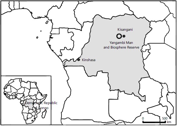
Study site: This study was conducted from June to July, 2018 in the Yangambi Biosphere Reserve, Yangambi, Democratic Republic of Congo. The history, climate, floristique composition of this reserve have widely been discussed by Jean de¹⁵. The study site is shown in Fig. 1.

Vegetation: The vegetation of the Yangambi Biosphere Reserve is part of the Guineo-Congolese Regional Center of Endemism. Its assessment has shown that there is a diversity of plant formations that can be explained both by the physical environment (the presence of several rivers in particular) and by the influence of man who has altered the habitats at different times. The vegetation of the Yangambi Biosphere Reserve is composed of undisturbed forests, secondary forests, mosaic forests, swamp forests and forest plantations¹⁵. Despite the anthropogenic pressure exerted on this Biosphere Reserve during the last years of war, almost ninety percent of it is now managed in a sustainable way by the National Institute for Agricultural Research (INERA), the owner of the site. There are about 737 ha of forest plantations, of which 600 ha are mainly composed of rubber cultivation and 137 ha are composed of different forest species imported from all the other provinces of the country. Several planting methods have been tested (layon method, Marineau method, dense placeau enrichment method and the white stock method). The oldest plantation dates from 1937¹⁶.

Fig. 1: Geographic location of the study area

Methodological approach of the study: A 90×90 m grid was installed in Lusambila mixed forest (Yangambi), then the coordinates of each selected tree species were recorded with a Geo-Explorer 7.0 Global Positioning System (GPS) and it’s the Diameter at Breast Height (DBH) measured. Tree’s name and family were also recorded. Additionally, soil samples were also collected at each tree location with a Koppechy cylinder at 10 cm depth and CO₂ emissions measured using a Vernier CO₂ gas sensor (Vernier, Beaverton, Oregon, United States of America) inserted in a 20 cm height and 15 cm diameter chamber (data not included). The sensor was hooked to LabQuest 2 (version 2.8.4), a standalone data logger with built-in graphing and analysis software 2 (version 2.8.4). The LabQuest 2 data logger was in turn connected to a laptop with Logger Pro 3 software. Soil temperature and moisture were measured using sensors connected to the data logger and the laptop (data omitted). Trees biomass was estimated with an allometric equation which relates the biomass of individual trees to easily obtainable non-destructive measurements, such as Diameter at Breast Height (DBH). The following allometric equation for the moist forest was used:

Y = 21.297-6.953(D)+0.740(D²)¹⁷

where, Y is biomass in kg/tree, D is DBH in cm and H is height in m.

Data on tree species and biomass were recorded in an Excel file and transferred into ArcGIS 10.3 where interpolated maps were produced using ARCGIS Geostatistical Analyst Extension. The distribution of tree species was predicted using seven geostatistical models: Inverse distance weighing, ordinary, simple and universal kriging, global and local polynomial interpolation and finally the Kernel interpolation methods.

A brief overview of spatial interpolation methods: Spatial interpolation is technique with the capability of producing prediction surfaces and also providing measures of the accuracy of these predictions. They are based on statistical models that include autocorrelation (statistical relationships among the measured points). They are used for data analysis in areas such as geography, atmospheric sciences, petroleum and mining exploration, environmental analysis, precision agriculture, fish and wildlife studies and many more. The ArcGIS software has an extension called ArcGIS-Geostatistical analyst containing these models. In this study, we tested 7 interpolation methods, namely: Local polynomial interpolation (LPI), Global polynomial interpolation (GPI), Inverse distance weighted (IDW), Simple (SK), Ordinary (OK) and Universal (UK) kriging and Kernel interpolation (KI). Local polynomial interpolation (LPI) method it is a deterministic interpolation method that adapts to many polynomials, each in specified overlapping neighborhoods. A first-order global polynomial fits a single plane through the data, a global second-order polynomial fits a surface with curvature, allowing surfaces to represent valleys, a global third-order polynomial allows two turns and so on. The local polynomial interpolation as well as other methods used in this study were extensively discussed by Kumar¹⁷.

RESULTS

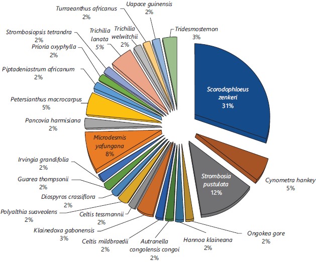
Floristic composition and specific dominance: The floristic composition of plant species is given in Fig. 2. It shows that a total of 60 individual trees, divided into 25 species and 35 families were selected (Table 1). The figure also shows that the species Scorodophloeus zenkeri was the most dominant with 31%, followed by Strombosia pustulata (12%) and Microdesmis yafungana (8%). Cynometra hankei, Petersianthus macrocarpus and Trichilia lanata each share a specific dominance of 5%.

Forest biomass: The mean for tree biomass was 2866.70 kg with a median value of 2597.20 kg. These 2 values are in the same range, meaning that biomass data approached normality. This wasis confirmed by lower skewness (0.9501) and kurtosis (0.5031) values. However, the coefficient of variation was 72.98% with a standard deviation of 2092.30, suggesting that forest biomass was highly variable across Yangambi Biosphere as expected.

Fig. 2: Repartition of plant species as function of their dominance

Table 1:

Trees species growth parameters

Species	Trees #	Families	Mean values -----------------------------------------------------------
			BA (m2)	DBH (cm)	BMS (kg)
Ongokea gore	1	Malvaceae	0.5808	85.99	8,125.20
Hannoa klaineana	2	Simaroubaceae	0.1017	35.99	1,190.50
Autranella congolensis	3	Sapotaceae	0.3614	67.83	4,889.50
Celtis mildibraedii	4	Cannabaceae	0.6246	89.17	8,777.20
Klainedoxa gabonensis	5	Irvingiaceae	0.1687	46.34	3,241.30
Celtis tessmannii	5	Cannabaceae	0.2876	60.51	3,815.60
Polyalthia suaveolens	7	Annonaceae	0.2065	51.27	2,651.60
Cynometra hankei Harms	8	Fabaceae	0.2302	54.14	3,191.70
Cynometra hankei	8	Fabaceae	0.1167	38.54	1,393.70
Diospyros crassiflora	10	Ebenaceae	0.2876	60.51	3,815.60
Cannabaceae	11	Cannabaceae	0.0147	13.69	100.3
Guarea thompsonii	12	Meliaceae	0.2697	58.6	3,557.40
Irvingia grandifolia	13	Irvingiaceae	0.204	50.96	2,615.30
Microdesmis yafungana	14	Pandaceae	0.1053	36.62	1,485.10
Pancovia harmisiana	15	Sapindaceae	0.046	24.2	460.5
Petersianthus macrocarpus	16	Lecythidaceae	0.1409	42.36	1,728.80
Petersianthus macrocarpus	17	Lecythidaceae	0.3962	71.02	5,676.20
Piptadeniastrum africanum	18	Fabaceae	0.1147	38.22	1,367.50
Prioria oxyphylla	19	Fabaceae	0.1675	46.18	2,100.10
Scorodophloeus zenkeri	20	Fabaceae	0.2242	53.42	3,039.70
Strombosia pustulata	21	Olacaceae	0.1106	37.53	1,585.90
Strombosiopsis tetrandra	22	Strombosiaceae	0.4589	76.43	6,320.10
Trichilia prieuriana	23	Meliaceae	0.1801	47.88	2,389.00
Trichilia welwitschii	24	Meliaceae	0.0645	28.66	696.2
Tridesmostemon claessensii	25	Sapotaceae	0.3513	66.88	4,741.90
Tridesmostemon claessensii	26	Sapotaceae	0.2275	53.82	2,951.60
Turraeanthus africanus	27	Meliaceae	0.0287	19.11	251.6
Uapaca guineensis	28	Phyllanthaceae	0.0231	73.57	5,822.80
BA: Basal area, BDH: Diameter at breast height and BMS: Biomass

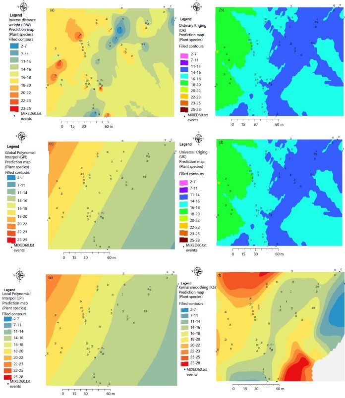
Predictive maps of the potential distribution of plant species: The predictive maps showing the spatial distribution of tree species are given in Fig. 3a-f for the different geostatistical models. These species distribution maps have several applications and the most common include estimating the ecological niche of species. An ecological niche can be described as an area within which a species can survive and reproduce depending on environmental factors which can be indirect or direct. These factors can influence the spatial distribution of species at three levels: (i) Limiting factors, which control the ecophysiology of the species (ii) Disturbances (natural or artificial, for example anthropogenic pressures) and (iii) Resources (food, water).

Inverse distance weighted method: The spatial distribution of tree species as predicted by the Inverse Distance Weighted (IDW) method is shown in Fig. 3a. The inverse distance weighted method predicted a high probability of the presence of Scorodophloeus zenkeri, Strombosia pustulata and Prioria oxyphylla in the Northwest. In the North-East and South-West, it shows an obvious under-representation of these three species. Furthermore, the map clearly shows a wider potential distribution of Microdesmis yafungana, Guarea thompsonii and Irvingia grandifolia in the Northeast, Petersianthus macrocarpus and Pancovia harmisiana in the Southeast Region.

Global polynomial interpolation method: The spatial distribution of tree species as predicted by the Global Polynomial Interpolation (GPI) method is shown in Fig. 3b. Overall, Fig. 4 shows a columnar clustered distribution of obliquely oriented species. The GPI predicted a high probability of the potential presence of species such as Pancovia harmisiana, Prioria oxyphylla, Petersianthus macrocarpus and Piptadeniastrum africanum in the center and a low probability of the presence of the species Scorodophloeus zenkeri, Strombosia pustulata, Strombosiopsis tetrandra and Trichilia lanata in the Northwest. The presence of species Celtis tessmanii, Klainedoxa gabonensis, Polyalthia suaveolens and Cynometra hankei is portrayed in Southeast of the map.

Fig. 3(a-f): Maps predicting the spatial distribution of trees species using geospatial models

Local polynomial interpolation method: The spatial distribution of tree species as predicted by the Local Polynomial Interpolation (LPI) method is showen in Fig. 3c. Along with the observation made in Fig. 3b, the map of the distribution of species by LPI predicts in the same way: A clustered distribution in a column of obliquely oriented species. The LPI predicts a high probability of the potential presence of species such as Pancovia harmisiana, Prioria oxyphylla, Petersianthus macrocarpus and Piptadeniastrum africanum in the center and Celtis tessmannii, Klainedoxa gabonensis, Polyalthia suaveolens and Cynometra hankei at the Southeastern end. On the other hand, it predicts a medium and low probability of the presence of the species Scorodophloeus zenkeri, Strombosia pustulata, Strombosiopsis tetrandra and Trichilia lanata at the Northwestern end.

Fig. 4(a-f): Maps predicting the spatial distribution of trees biomass using geospatial models

Ordinary kriging method: The spatial distribution of tree species as predicted by the Ordinary Kriging (OK) method is illustrated in Fig. 3d. The analysis of Fig. 3d showed that the potential distribution map of species by the OK method predicts a high probability of the presence of Scorodophloeus zenkeri, Strombosia pustulata and Prioria oxyphylla in the North-West and a small probability of the presence of Cynometra hankei, Diospyros crassiflora and Celtis mildbraedii in the extreme North-East. In the North-West and South-East, it shows an obvious representation of the distribution area of Pancovia harmisiana, Petersianthus macrocarpus and Piptadeniastrum africanum. Furthermore, the method predicts a clearly wider potential distribution of Microdesmis yafungana, Guarea thompsonii and Irvingia grandifolia and probably Pancovia harmisiana in the center of the area.

Simple kriging method: The simple kriging (SK) method predicted a map with a very high probability of the presence of Scorodophloeus zenkeri, Prioria oxyphylla and Strombosia pustulata. In addition, the northeastern, southern and central part of the prediction map was occupied by Pancovia harmisiana, Petersianthus macrocarpus and Piptadeniastrum africanum. Furthermore, it should be emphasized that the SK method did not predict the rest of the species present in the study area.

Universal kriging method: The spatial distribution of 3 species by the Universal Kriging (UK) method is illustrated in Fig. 3e. A quick analysis of Fig. 3e showed that the potential species distribution map made by UK is similar to the one for Ordinary Kriging (OK), in Fig. 3d. As previously observed, this map predicted a high probability of the presence of Scorodophloeus zenkeri, Strombosia pustulata and Prioria oxyphylla in the Northwest and a small probability of the presence of Cynometra hankei, Diospyros crassiflora and Cannabaceae in the far North-East. In addition, the probability of the presence of Scorodophloeus zenkeri, Strombosia pustulata and Prioria oxyphylla is much lower in the South-East, or even zero in the North-East. In the North-West and South-East, it shows an obvious representation of the distribution area of Pancovia harmisiana, Petersianthus macrocarpus and Piptadeniastrum africanum. Furthermore, the method predicts a clearly larger potential distribution of Microdesmis yafungana, Guarea thompsonii and Irvingia grandifolia and probably Pancovia harmisiana in the center of the area.

Kernel interpolation method: Results of the spatial distribution of tree species as predicted by the Kernel Interpolation (KI) method are shown in Fig. 3f. Analysis of this potential species distribution map shows high probability areas of the presence of Scorodophloeus zenkeri and Strombosia pustulata in the North-West, medium probability in the South-East and no probability of presence of these species in the North-East, in the center and in the South-West part, which would potentially be occupied by Pancovia harmisiana, Petersianthus macrocarpus and Piptadeniastrum africanum. Furthermore, the map predicts a potential spatial distribution of species like Ongokea gore, Hannoa klaineana, Autranella congolensis, Cannabaceae, Klainedoxa gabonensis, Celtis tessmannii, Polyalthia suaveolens, Cynometra hankei, Diospyros crassiflora, Cannabaceae, Guarea thompsonii, Irvingia grandifolia, Microdesmis yafungana and Pancovia harmisiana with high probability, exclusively in the eastern part and low probability towards in the South. Finally, the species distribution prediction map by the Kernel interpolation method shows a potential spatial distribution of Strombosiopsis tetrandra, Trichilia lanata, Trichilia welwitschii, Tridesmostemon claessensii, Turraeanthus africanus and Uapaca guineensis in the North-West and South-East.

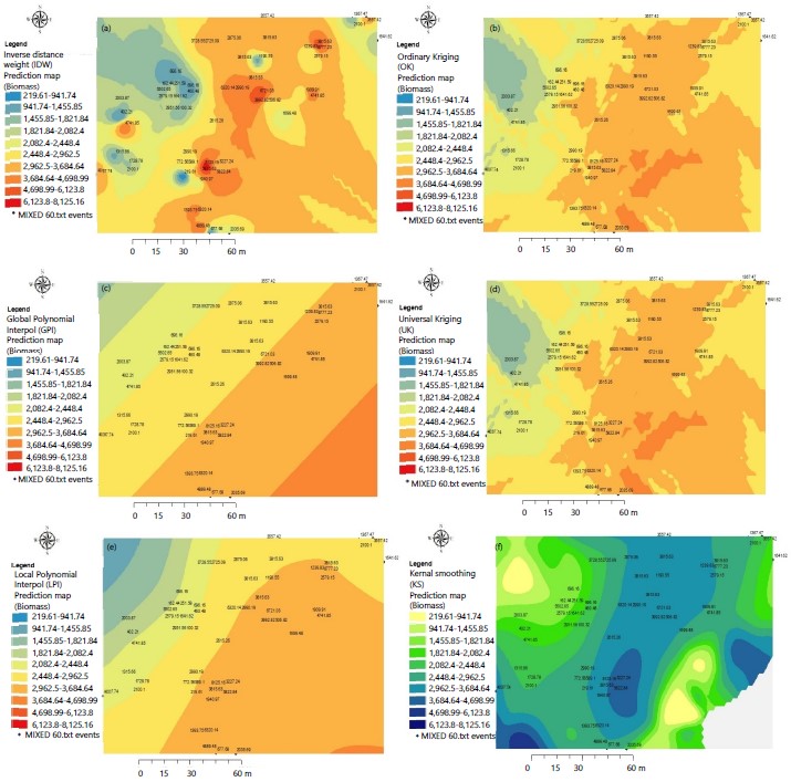
Predictive maps of potential distribution of trees biomass: The predictive maps showing the spatial distribution of trees biomass are given in Fig. 4(a-f) for the different geostatistical models. There were no instances where maps showing the spatial distribution of tree species matched those of trees biomass. Overall, the maps showed 2 zones, one with low biomass in the west side of the forest and high biomass in the east side, this regardless of the geostatistical model concerned. The inverse distance weighing (IDW) ordinary kriging (OK) and even universal kriging (UK) all depicted Ongokea gore, Celtis mildbraedii, Uapaca guineensis, Petersianthus macrocarpus, Autranella congolensis and Scorodophloeus zenkeri which in fact agreed with Table1. These were the species with the highest biomass. The local polynomial method (LPI), global polynomial (GPI and kernel smoothing method (SK) depicted Ongokea gore, Polyalthia suaveolens, Microdesmis yafungana, Pancovia harmisiana and Scorodophloeus zenkeri as species which highest biomass, but some of these species were placed in the South west and middle of the forest plot instead of the East of the plot as other geostatistical methods have showed.

DISCUSSION

Comparison between spatial interpolation methods for predicted tree species maps. The evaluation of these different spatial interpolation methods tested in this study is generally good, with the exception of the Global Polynomial Interpolation and the Local Polynomial Interpolation methods for which the 2 species prediction maps were almost identical Fig. 3(b-c). These two methods predicted a clustered columnar distribution of oblique oriented species, with a tendency to minimize the probability of the presence of dominant species such as Scorodophloeus zenkeri and Strombosiopsis tetrandra (Fig. 2). On the other hand, they also tend to predict these species only towards the North-East. It has been reported that when some species are more or less sampled than others, the prediction model may be influenced by the most common species or less represented one¹⁹. The comparison of potential species distribution maps from geostatistical methods showed that prediction maps produced by the Ordinary Kriging and the Universal Kriging methods were both similar. This similarity shows that they are both based on same statistical processes including autocorrelation, i.e. the statistical relationships between the measured points. The maps of favorable zones (of potential distribution) estimated by these models tended to be the most often optimistic¹⁸. For the rest, these methods seem to predict more or less correctly the zones of presence in the North-West of the area, a little less in the center and the East. The verification map (not included) of the spatial distribution of species therefore seems consistent with the prediction map of the distribution of species by the Simple Kriging method, more particularly for the species Scorodophloeus zenkeri in almost all geographical directions. This trend confirms the biogeographical history and environmental preferences of this species in these areas. In agreement with the other methods, the prediction maps of the distribution of species by the Kernel Interpolation method and that of Inverse Distance Weighting also seemed to corroborate with the reality of the verification map which shows a predominance of species such as Scorodophloeus zenkeri and Strombosiopsis tetrandra towards the North-West and towards the South and Cynometra hankei towards the East. In addition, among all of the methods tested, the Inverse Distance Weighting method gave rise to predictions centered around measured trees Fig. 3(a-f), while other methods in particular the simple, Universal and Ordinary Kriging methods, the Local and Global Polynomial Interpolation method have shown a tendency to predict areas of potential presence for larger species Fig. 3(b-f). The reasons for these differences can be attributed on the one hand to the profile of the presence of data, on the other hand to the distinct ecological characteristics of the species²⁰. The number and size of the grid can also have an impact on the methods and their predictive capacity¹². An intermediate number of presence cells, distributed in a homogeneous manner and fully included in a restricted distribution area leads to a good prediction of the geographical distribution of species. On the contrary, for an intermediate or large sample, with places of higher prevalence and wide geographical distribution, the models tend to make conservative or erroneous predictions, contrary to a small sample and an intermediate distribution area, allowed to obtain a good prediction of the potential distribution area. Furthermore, as said earlier, several studies have shown that different prediction methods can lead to different results²¹ because these methods are sensitive to the available data and the mathematical functions used¹⁴. Forest biomass showed an East-West distribution with trees with the highest biomass on the eastern portion of the forest. This may be due to environmental factors influencing forest growth. It is recommending that the study be repeated for a larger area (at least 150×150 m). The number of trees to be measured should be increased, for example doubled, but the spatial interpolation methods can be limited to three: Inverse distance weighing, Ordinary kriging and Universal kriging if variograms can be fitted.

CONCLUSION

The present study aimed to determine the most appropriate and efficient methods for the prediction of the geographical distribution of tree species and their biomass in the Yangambi Biosphere Reserve. To achieve this, a systematic inventory of the selected species was carried out using Global Positioning System (GPS) and tree parameters measurements. From these data, the prediction maps were made with seven spatial interpolation methods. Although, these models are promising, it would be desirable that this study be repeated over time and in several places to determine the best models to be used in our region/country for a better understanding of the spatial distribution of forest tree species and their biomass.

SIGNIFICANCE STATEMENT

Knowledge of tree species distribution and their biomass estimates is critical for monitoring forest carbon storage and for strategic forest management. Unfortunately, measuring tree parameters to obtain such information can be a time-consuming process that may require a great deal of manpower. Therefore, randomly taking a few measurements of tree parameters to calculate the biomass and predicting the rest of these parameters can help to quickly identify forest areas of interest in terms of tree biomass management. Therefore, this study provides an opportunity to quickly obtain the needed information to improve forest management operations.

REFERENCES

1. Vermeulen, C., É. Dubiez, P. Proces, S.D. Mukumary and T.Y. Yamba et al., 2011. Land issues, exploitation of natural resources and local community forests on the outskirts of Kinshasa, DRC [In French]. Biotechnol. Agron. Soc. Environ., 15: 535-544.
2. Tyukavina, A., M.C. Hansen, P. Potapov, D. Parker and C. Okpa et al., 2018. Congo Basin forest loss dominated by increasing smallholder clearing. Sci. Adv., 4.
3. Aleixo, I., D. Norris, L. Hemerik, A. Barbosa, E. Prata, F. Costa and L. Poorter, 2019. Amazonian rainforest tree mortality driven by climate and functional traits. Nat. Clim. Change, 9: 384-388.
4. Pretzsch, H., R. Grote, B. Reineking, T. Rotzer and S. Seifert, 2008. Models for forest ecosystem management: A European perspective. Ann. Bot., 101: 1065-1087.
5. Thammanu, S., D. Marod, H. Han, N. Bhusal and L. Asanok et al., 2021. The influence of environmental factors on species composition and distribution in a community forest in Northern Thailand. J. For. Res., 32: 649-662.
6. Guisan, A. and W. Thuiller, 2005. Predicting species distribution: Offering more than simple habitat models. Ecol. Lett., 8: 993-1009.
7. Cardoso, P., T.L. Erwin, P.A.V. Borges and T.R. New, 2011. The seven impediments in invertebrate conservation and how to overcome them. Biol. Conserv., 144: 2647-2655.
8. Gatti, R.C., P.B. Reich, J.G.P. Gamarra, T. Crowther and C. Hui et al., 2022. The number of tree species on earth. Proc. Natl. Acad. Sci., 119: e2115329119.
9. Robertson, M.P., G.S. Cumming and B.F.N. Erasmus, 2010. Getting the most out of atlas data. Divers. Distrib., 16: 363-375.
10. Pearson, R.G., W. Thuiller, M.B. Araujo, E. Martinez-Meyer and L. Brotons et al., 2006. Model-based uncertainty in species range prediction. J. Biogeogr., 33: 1704-1711.
11. Araújo, M.B. and M. New, 2007. Ensemble forecasting of species distributions. Trends Ecol. Evol., 22: 42-47.
12. Zakeri, F. and G. Mariethoz, 2021. A review of geostatistical simulation models applied to satellite remote sensing: Methods and applications. Remote Sens. Environ., 259: 112381.
13. Guisan, A. and N.E. Zimmermann, 2000. Predictive habitat distribution models in ecology. Ecol. Model., 135: 147-186.
14. Phillips, S.J., R.P. Anderson and R.E. Schapire, 2006. Maximum entropy modeling of species geographic distributions. Ecol. Modell., 190: 231-259.
15. Jean de, H., 1952. Soils, Paleosols and Ancient Desertifications in the North-Eastern Sector of the Congo Basin. National Institute for the Agronomic Study of Congo (INEAC), Congo, pages: 168.
16. Brown, S. and A.E. Lugo, 1984. Biomass of tropical forests: A new estimate based on forest volumes. Science, 223: 1290-1293.
17. Kumar, A., S. Maroju and A. Bhat, 2007. Application of ArcGIS geostatistical analyst for interpolating environmental data from observations. Environ. Prog., 26: 220-225.
18. Whittaker, R.J., M.B. Araújo, P. Jepson, R.J. Ladle, J.E.M. Watson and K.J. Willis, 2005. Conservation biogeography: Assessment and prospect. Divers. Distrib., 11: 3-23.
19. Barbet-Massin, M., F. Jiguet, C.H. Albert and W. Thuiller, 2012. Selecting pseudo-absences for species distribution models: How, where and how many? Methods Ecol. Evol., 3: 327-338.
20. Hanberry, B.B., H.S. He and B.J. Palik, 2012. Pseudoabsence generation strategies for species distribution models. PLoS ONE, 7: 0044486.
21. Schure, J., F. Pinta, P.O. Cerutti and L. Kasereka-Muvatsi, 2019. Efficiency of charcoal production in Sub-Saharan Africa: Solutions beyond the kiln. Bois. Forets Des Tropiques, 340: 57-70