A Computer Vision-Based Approach to Estimate Disease Severity for Field-Taken Wild Blueberry Images

Received 27 Mar, 2024

Accepted 24 May, 2024

Published 30 Jun, 2024

Background and Objective: In contrast with the laboratory environment, it is challenging to quickly and accurately rate disease severity in real farming conditions for high-density crops like blueberries. In field-taken images, the target diseased organs are usually shaded, interfered, occluded and backgrounded by other plants or plant parts, which are often irrelevant to severity estimation. This study aimed to develop and validate a computer vision-based severity estimation algorithm for mummy berry disease, which enables labor-free severity estimation with high accuracy and applicability in real farming conditions. Materials and Methods: This study developed a fast and accurate severity estimation algorithm for wild blueberry diseases by utilizing computer vision-based techniques. Firstly, this study employed a novel deblurring process using defocus estimation to effectively remove blurred parts so that the diseased and healthy target organs can be separated from the irrelevant background. This method was also enhanced by using adjustable parameter settings so that low-quality images such as those without clear focus could be properly handled. Secondly, by converting RGB features into HSV space followed by bootstrap forest modeling, diseased organs can be automatically segmented and then the severity can be estimated by calculating the ratio of total diseased pixels to the total pixels excluding background. Results: This step can effectively alleviate the negative impact of light variations such as shading on diseased organs. Verifications and experiments conducted on 400 disease images demonstrated that this approach can effectively identify diseased and healthy plant organs and make an accurate estimation with less than an average 5% relative error across different levels of background complexity and image quality. Conclusion: The method can serve as an auto-labeling tool to automatically rate the disease severity for field-taken images, on which severity estimation deep learning models can be trained without the limitation of data scarcity.

INTRODUCTION

Wild lowbush blueberry (Vaccinium angustifolium Aiton) is a species of blueberry native to Northeastern North America¹, where approximately 100 million kg of wild blueberries are produced annually². Due to the high economic value of blueberries and the increasing threat of diseases, issues related to blueberry diseases need to be addressed. Common blueberry diseases are numerous, with the most significant being mummy berry disease³. This disease can occur at different stages of blueberry growth, posing a significant threat to the yield and quality of blueberries^4,5. The application of computer vision methods for automated assessment of the severity of blueberry diseases can help understand disease spread, estimate threat levels and thus provide information for developing targeted prevention and control strategies.

The severity of plant diseases, defined as the proportion of plant organs (e.g., leaves) with evident disease symptoms to the total plant organs, is a critical quantitative metric for many diseases⁶. It serves as the basis for deciding the type and quantity of treatments when undertaking disease prevention and control measures⁷. Timely and accurate detection of the severity of plant diseases is particularly important for farmers, as it helps them make effective decisions to protect crops from secondary infection and reduce economic losses. Traditional methods for assessing crop disease severity typically encompass two approaches: Expert scoring and automated assessment⁸. Expert scoring involves specialists evaluating the extent of crop disease based on a predefined assessment indicator system⁹. Automated assessment primarily relies on hyperspectral remote sensing technology¹⁰. In recent years, there have also been methods based on image processing and deep learning for disease severity assessment^11,12. Image processing often involves rating the proportion of the diseased area to the healthy area to estimate severity. Deep learning methods mostly treat disease grading as a classification task, training models with input data that include different levels of disease severity¹³.

Regardless of many computer vision-based approaches taken to assess the disease severity of high-density crops like wild blueberries, two problems arise. The first problem is how to eliminate interferences from irrelevant objects and accurately delineate the affected and healthy regions from images? A blueberry plant image captured in real-farming conditions typically comprises three categories of objects: One being the infected organs, the second being the healthy organs and the third being other parts unrelated to severity assessment. The irrelevant parts include unrelated backgrounds like the sky and trees, as well as other blueberry plants with backgrounds resembling disease symptoms. In this scenario, the overlap and obstruction of these unrelated elements are the primary factors affecting interference recognition and computation, making it crucial to effectively remove them during the identification process.

Another problem is how to deal with the color variation in disease visual characteristics caused by uncontrollable natural light conditions, enabling accurate identification. Diseases typically exhibit distinct color characteristics compared to healthy portions, thus leveraging this trait for extraction of the infected parts is feasible. However, the visual characteristics of diseased areas in the image are highly sensitive to changes in brightness, which, unlike controlled laboratory conditions, are inevitable in field conditions. For the same ailment, significant color differences will be reflected under different lighting conditions. This poses significant difficulties for machine vision-based disease extraction methods. Hence, an appropriate disease feature extraction method holds paramount importance for the accurate estimation of disease severity.

The first problem can be solved by removing irrelevant content from the image before extracting the diseased organs. In general, images taken for disease severity estimation purposes, have their focus on the diseased organs surrounded by healthy parts of the stem in the blueberry plant. Other areas, apart from these, are usually irrelevant and relatively blurred, which can be removed so that the infection severity can be accurately estimated. Defocus estimation plays a significant role in various computer vision and computer graphics applications, including depth estimation, image quality assessment, image deblurring and refocusing¹⁴. Its purpose is to estimate the depth of field information for foreground and background objects from the image¹⁵.

Utilizing defocus estimation allows differentiation between the blurred and non-blurred portions of the image, which benefits the removal of interfering factors and leads to a more accurate estimation¹⁶. However, the defocus estimation process comes with numerous challenges¹⁷, such as depth information loss, blur and distortion, lighting variations, multiscale issues, noise interference and motion blur, making it difficult to perform defocus estimation on images captured in outdoor settings¹⁸. One typical example is that the degree of blur might be uneven across all the images taken for severity estimation considering the effects of different shooting habits and constraints in the field¹⁹. Therefore, how various degrees of blur can be properly handled to generalize its applicability in real-farming conditions is critical.

Aside from the removal of blurred interference, a lot of research efforts have been devoted to the work of extracting diseased regions. Infected blueberries were physically observed by experts and researchers, a process that was both labor-intensive and costly²⁰. With the increasing application of deep learning methods in agriculture, disease identification in crops not only saves labor in feature engineering but also achieves high accuracy in many real field conditions. While deep learning can retrain efficient and accurate models based on extensive data collection, this process demands significant time and effort for accurate data labeling, i.e., the fidelity to rating the degree or severity²¹. Therefore, attention has gradually shifted back to conventional computer vision methods to avoid extensive manual labeling. Many histogram equalization-based methods have been reported by researchers^22-24in which the diseased parts of the plant can be segmented by means of image processing using feature extraction and classification techniques such as self-organizing feature maps, back-propagation algorithms, SVMs. These solutions work well for images taken in a controlled lab environment but are sensitive to light variations in real-farming conditions²⁵. Therefore, how light variations in real field conditions can be sufficiently suppressed to minimize their effects on severity estimation is crucial.

This study aimed to develop and validate a computer vision-based severity estimation algorithm for mummy berry disease, which enables labor-free severity estimation with high accuracy and applicability in real farming conditions. The study proposed a novel deblurring technique using defocus estimation based on the Gaussian gradient ratio to remove blurred areas that are irrelevant to severity estimation, so that accuracy can be promoted by rating relevant only elements and robustness to various degrees of blurriness can be achieved by using dynamic parameterization. Then proposed a bootstrap forest method to learn the segmentation parameters in HSV color space so that the effects of light variation on disease feature extraction can be minimized. This approach not only provides an effective and accurate severity estimation module for field surveillance AI systems, but also can serve as an auto-labeling tool for automatic rating of disease severity for field-taken images, on which severity estimation deep learning models can be trained without the limitation of data scarcity.

MATERIALS AND METHODS

Data collection
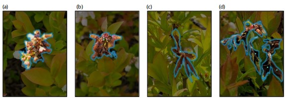
Sampling location and method: The study was carried out from May, 2023 to December, 2023. Sample images of diseased wild blueberry plants were taken at the experimental stations of the University of Maine Blueberry Hill Farm (BBHF) in Jonesboro, Maine, USA (Latitude: 67°38'53"W, Longitude: 44°38'44"N). Photographs were taken from multiple angles using a digital camera with a resolution of (1280 to 3480) x1080p. The shooting distance was fixed at 1 meter and images were required to focus on diseased lesions on leaves or flowers of a blueberry plant (Fig. 1a-b).

Fig. 1(a-b): Example field images focused on diseased blueberry (a) Leaves and (b) Flowers

Fig. 2(a-d): Sample images of mummy berry disease on (a-b) Flowers and (c-d) Leaves Light (a, c) and severe (b, d) symptoms are visually marked by a blue contour line

Dataset description: The image dataset primarily comprises various affected parts of blueberry plants with mummy berry disease. Mummy berry disease is caused by the fungal pathogen Monilinia vaccinii-corymbosi²⁶ and is one of the major diseases of blueberries. The disease causes irregular dark brown spots and grayish-white mold on parts of blueberry flowers, leaves, fruits and stems (Fig. 2a-b). Symptoms usually appear early in the season with a general brown coloration around the major leaf veins²⁷. As the disease progresses, leaves, new shoots, buds and flowers may wilt, turn brown and drop (Fig. 2c-d). To establish the sample image dataset, over 400 images were captured specifically focusing on blueberry plants affected by mummy berry disease.

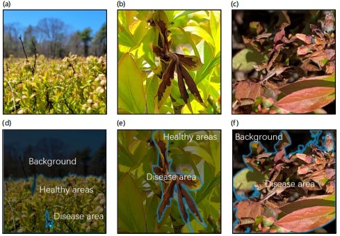
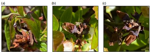
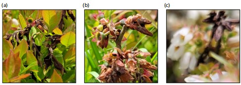
Typical images taken for blueberry disease severity evaluation have two main features that affect estimation, i.e., (1) Effects of background and light conditions and (2) Image quality. As a density crop, many elements in the images are irrelevant to the severity estimation of the target plant and need to be removed: (1) Background area including sky, trees, etc. (Fig. 3a); (2) Other blueberry plants that can not be counted for rating the target plant (Fig. 3b) and (3) Backgrounds with similar characteristics resembling the disease (soil, fallen leaves and etc. Fig. 3c). The three components in the example image (Fig. 3a-c) are shown respectively in figures (Fig. 3d-f). In field rating scenarios, natural light is not controllable and subject to change. Even with the same symptom on the same plant, light variations can significantly change the visual traits of the diseased lesions (Fig. 4a-c), which is a major barrier to feature extraction by computer vision techniques. In reviewing the field-collected images, a small portion of them shows various degrees of blurriness, as shown in Fig. 5a-c where three typical levels of blurriness (accurately focused, slightly out-of-focus and severely out-of-focus images) were presented. This phenomenon is common due to varying shooting distances and instabilities during focusing²⁸.

Fig. 3(a-f): Elements within the field taken images irrelevant to severity estimation, (a) Background (e.g., sky, trees), (b) Other blueberry plants, (c) Background resembling disease symptoms and (d-f) Close-ups of irrelevant parts and the diseased area in a-c

Fig. 4(a-c): Visual traits of the same symptom of mummy berry disease affected by different lighting conditions, (a) Sufficient light, (b) Partially shaded and (c) Severely shaded

Fig. 5(a-c): Typical blurriness variations in field-collected images, (a) Accurately focused image (high quality), (b) Slightly out-of-focus images and (c) Severely out-of-focus images (low quality)

Fig. 6: Overview of the proposed image process and disease severity estimation approach with an example. Steps, methods and examples are provided

Severity estimation
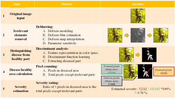
Method overview: The proposed approach takes a field-sampled image focusing on disease as an input, then a deblurring process is applied to remove irrelevant elements in the image. The deburring process includes three steps, which are (1) Blur edge identification, (2) Defocusing blur and (3) Defocusing map interpolation. This process can effectively suppress interferences from the background and other graphical elements irrelevant to disease evaluation. Then, a bootstrap forest model is applied to extract the diseased part from the healthy part after the irrelevant elements are removed. This step requires feature representation of diseased and healthy parts in color space, from which a decision boundary and its parameters can be learned to accurately separate the diseased part from the healthy background. This process is done on the whole dataset to gain a statistically robust parameter estimation for the decision boundary. Once the disease extraction is done, the number of pixels of the diseased part and the healthy part can be counted, respectively. Finally, the ratio of the disease pixels to the total area except for the irrelevant elements is calculated as the estimation of disease severity. The whole process is illustrated in Fig. 6 and further clarified using an example.

Removal of irrelevant elements: Statistical evidence (unpublished data and the dataset established in this study) showed that images taken for disease severity estimation share the common feature that the diseased organs and their healthy counterparts are usually focused while other parts are relatively blurry. Therefore, removing the blurry parts, i.e., the process of deblurring, can eliminate the interference from irrelevant elements in the image in severity estimation. The process of deblurring consists of three main steps: (1) Establishing the defocus model, (2) Defocus blur estimation and (3) Defocus map interpolation.

Defocus modeling (f): This study calculates the defocus blur at the edges, focusing specifically on edge locations. Given that the step edge is the predominant edge type in natural images, our study exclusively addresses step edges. An ideal representation of a step edge can be conceptualized as²⁹:

f(x) = Au(x)+B

(1)

The step function is denoted by u(x), where, A and B represent the amplitude and offset of the edge, respectively. It is important to note that the edge is positioned at x = 0.

Fig. 7(a-b): Concepts of focus and defocus within thin lens model, (a) Focus and defocus for thin lens model and (b) Diameter of CoC c as a function of the object distance d and f-stop number N given df = 500 mm and df = 80 mm

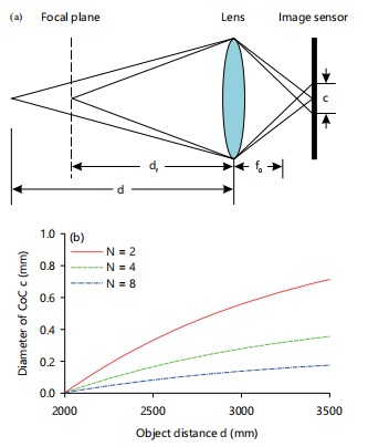
Assuming adherence to the thin lens model, focus and defocus follow certain principles. Specifically, when an object is positioned at the focal distance d_f, the rays emanating from a particular point on the object converge onto a single sensor point, rendering the image sharp. Conversely, rays from a point on another object located at distance d will reach multiple sensor points, leading to an image characterized by blurriness. The nature of the blur is contingent on the shape of the apture and is termed the circle of confusion (CoC). The diameter of the CoC serves as a descriptor for the degree of defocus and can be expressed as³⁰:

(2)

In the given context, f₀ denotes the focal length, while N represents the stop number of the camera. Figure 7a-b visually depicts the concepts of focus and defocus within the thin lens model, specifically highlighting the variation in the diameter of the circle of confusion concerning both the object distance (d) and the stop number (N). This illustration assumes fixed values for the focal length (f₀) and focal distances (d_f). It is apparent from the diagram that the diameter of the circle of confusion (CoC), denoted as c, follows a non-linear, monotonically increasing pattern in relation to the object distance d.

The representation of defocus blur involves modeling it as the convolution between a sharp image and the point spread function (PSF). The PSF is commonly approximated using a Gaussian function, denoted as g(x,σ), where the standard deviation σ = kc serves as a measure of the defocus blur extent, directly proportional to the diameter of the circle of confusion (CoC) c. The resulting formula for a blurred edge i(x) is then derived as³¹:

(3)

Fig. 8: Overview of blur estimation approach

Here ⊗ and ∇ are the convolution and gradient operators, respectively. The black dash line denotes the edge location

Defocus blur estimation: For blur estimation, an edge undergoes re-blurring with a predetermined Gaussian kernel initially (Fig. 8). Subsequently, the ratio between the gradient magnitude of the original step edge and its re-blurred counterpart is computed. This ratio is determined as the maximum value at the edge location. By utilizing this maximum value, the extent of defocus blur determined at the specific edge location.

To enhance clarity, blur estimation method was presented initially for the 1D case and subsequently extended it to the 2D image scenario. The gradient of the re-blurred edge is then expressed as³²:

(4)

where, represents the standard deviation of the re-blur Gaussian kernel, also known as the re-blur scale. The ratio of gradient magnitudes between the original and re-blurred edges was then expressed as³²:

(5)

A proof demonstrates that the ratio attains its maximum at the edge location (x=0) and the maximum value is determined by Canny³³:

(6)

Based on the analysis presented in Eq. 4 and 6, it becomes evident that the edge gradient is contingent on both the edge amplitude A and the blur amount s. However, when considering the maximum of the gradient magnitude ratio R, the influence of the edge amplitude A is nullified and the dependency is solely on and . Therefore, leveraging the maximum value of R at the edge locations, we can calculate the unknown blur amount s using³³:

(7)

In the case of 2D images, the process of blur estimation is analogous. Re-blurring is achieved using a 2D isotropic Gaussian kernel and the computation of gradient magnitude unfolds as follows³³:

(8)

The notation ∇i_x and ∇i_y denotes gradients along the x and y directions, respectively. This approach fix σ₀ = 1 for re-blurring and utilize the Canny edge detector for edge identification. Another assumption is a linear camera response curve.

The estimation of blur scales takes place at each edge location, resulting in a sparse depth map represented by

Defocus map interpolation: With the obtained sparse defocus map, denoted as in the previous step, this approach involves extending defocus blur estimates from edge locations to the entire image, which resulted in a comprehensive depth map This entails determining a defocus map, denoted as d(x), that closely approximates the sparse defocus map d(x) at each edge location. Additionally, the study aims to align defocus blur discontinuities with image edges. For these tasks, edge-aware interpolation methods are commonly employed^34,35. This case specifically utilize the matting Laplacian³⁶ for defocus map interpolation. Formally, the depth interpolation problem is cast as the minimization of the following cost function³⁰:

(9)

In this context, and d denote the vector representations of the sparse defocus map and the complete defocus map d(x), respectively. The matrix L represents the matting Laplacian, while D is a diagonal matrix with D_ii equaling 1 if pixel i is at an edge location and 0 otherwise. The scalar l serves as a balance parameter, determining the trade-off between fidelity to the sparse depth map and the smoothness of interpolation. The (i, j) element of L is formally defined as³⁰:

(10)

The expression involves the Kronecker delta, denoted as δ^ij, where U_ξ is a 3*3 identity matrix. The μ_k and σ_k represent the mean and covariance matrix of colors within the window ω_k. The I_i and I_j refer to the colors of the input image I at pixels i and j, respectively. The parameter ε serves as a regularization factor and |ω_k| denotes the size of the window ω_k. For a more in-depth derivation of Eq. 10, readers are directed to³⁶.

The optimal solution for d can be obtained by solving the following sparse linear system³⁰:

(11)

The default setting for λ is 0.005 to impose a soft constraint on d, aiming to enhance the accuracy of blur estimation by refining minor errors. This soft matting approach has also been employed in previous studies^37-38 to address challenges related to dehazing and spatially variant white balance issues.

Sensitivity of parameter λ: As previously reported by Zhuo and Sim³⁹, the default setting of parameter λ works well for sharp images but might not be suitable for images suffering various degrees of blurriness. This phenomenon is common due to varying shooting distances and instabilities during focusing but might negatively affect the deblur process and consequently cause incorrect segmentation of diseased parts. Field-collected image dataset also showed that a small portion of them had various degrees of blurriness (Fig. 5). Therefore the study investigated how this parameter is related to blur estimation and tried to find the appropriate setting of λ to cope with this uncertainty in field-collected images.

Distinguishing disease from the healthy part
Feature representation in color space: In the RGB color model, the color of each pixel in a color image is expressed as a triplet (R, G, B), each component of which is extracted as a value between 0 and 255. In order to alleviate the effects of light changes in real farming conditions on identification results, here will also discuss another type of color space, namely the HSV color space. The HSV color space is a way of mapping the RGB color space into a three-dimensional inverted cone. It describes color attributes through three parameters: Hue (H), Saturation (S) and Value (V). The Hue (H) is identified by an angle from 0-360°, where red is at 0°, green is at 120° and blue is at 240°. Saturation (S) represents the purity or intensity of color. The higher the saturation, the more pure and intense the color; conversely, when the saturation is lower, the color tends towards gray or white, that is, more white components are mixed in. The Value (V) is used to measure the brightness of the color. The process of converting from the RGB color space to the HSV color space is shown in the following equations:

(12)

(13)

V = Max (R, G, B)

(14)

Therefore, the feature of each pixel was represented as six components, i.e., R, G, B, H, S and V, in both RGB and HSV color space. Then each pixel was labeled as either diseased (1) or healthy (0) for each image from the previous step because it contained only diseased and healthy elements. Considering the dimensions of an image in this study is 600*600 pixels, there were 360,000 data points, each of which had 6 components of color features and the corresponding diseased label. Manually segmented the diseased area from the healthy area for 200 images (randomly selected from the whole dataset, see description in section 2.1.2), so that the dataset of color features with the corresponding diseased label had 360,000*200 = 72,000,000 data points in total. Since it was a huge dataset and not efficient for model training, randomly selected 5% points from each image based on a uniform sampling method, so the total data points were still 360,000.

Methods for automatic differentiation between diseased and healthy parts: Given the above dataset with color feature and the corresponding segmentation label, the study conducted a supervised machine learning process to train a bootstrap forest⁴⁰ model in JMP Pro (Analyze->Predictive Modeling). The bootstrap forest can learn the decision boundaries between the diseased and healthy pixels as a function of the nonlinear combination of color components in either RGB or HSV space. This nonparametric model used instead of the parametric model, e.g., Linear Discriminant Analysis (LDA)⁴¹ because based on exploratory data analysis, it is found the distribution of some color components was not satisfactory to the model assumption. The 5-fold cross validation method⁴² was used to train and validate the bootstrap forest model. Once the prediction accuracy of the bootstrap forest model reaches an acceptable level, it then can be used as a classifier to differentiate diseased parts from healthy parts in the color space.

Severity estimation: Once the type of each pixel, i.e., either diseased or healthy, in an image can be classified, the area of diseased and healthy parts can be calculated by counting the total number of pixels in each corresponding area. Then the ratio of diseased area to the total area of diseased and healthy area was calculated as the estimation of disease severity. The pixel-counting approach was employed based on two considerations. The first one was to avoid complexity in dealing with irregular and scattered shapes of plant organs, in previous studies their numbers need to be accurately recognized and counted but may face big challenges in processing complex images taken in real farming conditions. The second one was to reduce the computational complexity in situations with possible occlusions among a large number of organs and complex backgrounds, which is often necessary in real-field applications.

Experiments
Experimental settings: This study conducted two sets of experiments to verify the proposed method and its effectiveness and to test the accuracy of severity estimation on the whole blueberry disease dataset. In the verification of the proposed methods, firstly, detailed each step of the deblurring technique with examples to test the effectiveness of removing irrelevant objects in the image for accurate estimation. Specifically, tested the impact of various degrees of blurriness in images on disease region extraction and investigated how changes in parameter λ would alleviate this impact; Secondly, demonstrated the robustness of automatically learning parameters for differentiating diseased parts from healthy parts in the color space.

Beyond the verification process, the validation process was taken on the whole mummy berry disease dataset with 400 images to statistically demonstrate its effectiveness. The first validation was to compare the relative error between methods with or without the process of deblur. The second validation was to compare the relative error between disease discrimination between HSV and RGB color space.

Evaluation metrics
Ground truth labeling: In this study, the labeling of ground truth was done by computer graphic tools and supervised by blueberry experts. For each image, the contour line of different types of regions, such as diseased, healthy parts and background as well as other irrelevant plants were identified manually by using the built-in image information panel of photoshop software⁴³. Photoshop allows obtaining essential information about the dimensions of objects in the input image, including their length, height and area by means of pixel counting. The pixel counting for the diseased region requires manual delineation. After manually marking the regions, their types and areas were recorded into the dataset. Based on the information extracted by Photoshop, the ratio of the total number of pixels in the diseased area to the total pixels in the focused plant area (excluding background and irrelevant objects) was then updated as the ground truth. The 400 images of the whole blueberry disease dataset (as described in section 2.1.2) were annotated and their ground truth of disease severity was recorded.

Error of estimation: Relative error (RE) and Root Mean Square Error (RMSE) were used as evaluation metrics for all the experimental results in this study. The lower the value of these two metrics, the better the experimental effect will be. The RE is used to explain the relative error between the predicted value and the true value. The RMSE is used to explain the sample standard deviation between the predicted value and the true value:

(15)

(16)

In the above equation, n is the number of samples, Y_i is the actual value (ground truth) of disease severity and X_i is the predicted value obtained by our method.

RESULTS AND DISCUSSION

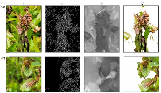
Verification of deblurring effectiveness: Figure 9 demonstrated the verification of irrelevant elements removal and gave two examples i.e., mummy berry disease on flowers (Fig. 9a), mummy berry disease on leaves (Fig. 9b). The deblurring process (see description in section 2.2.2) was performed on the two examples and the results were given in column II, III and IV in Fig. 9a,b. The sparse defocus map in column II showed the edge of the corresponding input image. It can be observed that the edge map modeling the clear parts of the input image was relatively dense, which indirectly reflects the effectiveness of our method in blur estimation. Interpolation on the edge map showing column II yielded the full defocus image, denoted as column III, representing the depth information of the image. The higher the grayscale, the clearer the relevant part including both diseased and healthy plant organs. This result clearly shows that the proposed deblurring method can effectively separate the focused blueberry plants from the background irrelevant to disease. Finally, the RGB restoration was performed on the higher grayscale regions, resulting in the recovered full-dispersion map shown in column IV. By comparing with the depth information in the full defocus map (column III), it demonstrated that this method can effectively preserve the clear parts of the image, achieving the goal of removing irrelevant parts. Additionally, it is worth noting that the proposed method can successfully remove irrelevant content in the mummy berry disease, demonstrating its applicability and robustness.

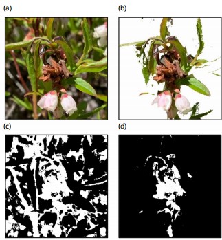
Figure 10 also quantitively compared the accuracy of disease severity estimation between the approach using the deblurring process and the approach where the disease extraction process (see section 2.2.3) was directly applied without deblurring. The ground truth of disease severity of the sample image (Fig. 10a) was 8.83%. The de-blurred image is shown in Fig. 10b. The severity estimated without using the deblurring process was 38.8% (Fig. 10c), which was much higher than the estimation applying deblurring (Fig. 10d), the latter estimated as 8.40% with only a relative error of 4.87%.

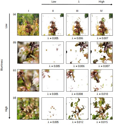
In addition, to address the problem of the inability to extract diseased parts from images with different levels of blurriness, this study investigated how parameter λ in equation 11 is related to blur estimation and tried to find the appropriate setting. This step is important to cope with uncertainties of sharpness (quality) in field-collected images⁴⁴. As shown in Fig. 11, for input images with different levels of blurriness (Fig. 11a-d), using a fixed λ value of 0.005 (suggested by Huihui et al.⁴⁵ and Yi and Eramian⁴⁶ as mentioned earlier), did not adequately preserve the diseased areas (Fig. 11II). That is mainly because changes in blurriness could affect defocus modeling. In the sensitivity analysis on parameter λ, for different levels of blurriness, find a suitable λ value that allows for the removal of relatively blurry areas in the image while preserving the diseased regions (Fig. 11III-IV). From this analysis, a positive correlation between the level of blurriness and λ is highly likely, i.e., the larger the λ value, the more accurately the non-diseased areas in the blurry image are removed and the more accurately the diseased areas are preserved.

Fig. 9(a-b): Defocus map estimation on two sample images, (a) Mummy berry disease on flowers and (b) Mummy berry disease on leaves I: Input image. II: Sparse defocus map. III: Full defocus map and IV: Recovered full-dispersion map

Fig. 10(a-d): Display of the impact of de-blurring on the effectiveness of disease extraction, (a) Original image, (b) De-blurred image, (c) Disease extraction performed on the original image and (d) Disease extraction performed on the de-blurred image

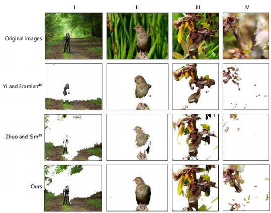
This study compared the effectiveness of deblurring of our method with the two representative methods, e.g., Yi and Eramian⁴⁶ using sharpness and Zhuo and Sim³⁹ using depth information. This comparison was conducted on four original images (Fig. 12), in which the first and second (Fig. 12 I-II) were incorporated from their papers and the third and fourth (Fig. 12III-IV) were from blueberry dataset representing high- and low-quality images. The detailed differences were embodied in the completeness of deblurring and stability in dealing with image quality variations.

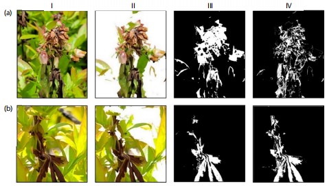
Verification of disease extraction effectiveness: First, disease extraction effectiveness was compared between methods using HSV and RGB color space after deblurring. In this comparison, two typical symptoms of mummy berry disease were considered, which were: Mummy berry disease on flowers and mummy berry disease on leaves, as shown in scenarios A and B in Fig. 13. Visual comparisons between the two color spaces were presented in column III and IV, which demonstrated that the extraction under RGB color space was more likely to confuse the regions with similar colors and the rest of the parts were not much different from those selected by the HSV method. Qualitatively, extraction under RGB color space incorrectly included healthy organs and lost diseased regions with similar color. One obvious finding was that extraction using RGB lost many pixels in the diseased area because their value in R channel became similar to those in the healthy area due to the changes in light (or shading). This caused many empty pixels in the diseased area underestimating the severity. Quantitative comparisons also showed that the relative error of extraction using HSV were almost 10 times lower than using RGB. The former achieved 4.32 and 3.78%, respectively, whereas the latter were 36.3 and 26.2%.

Fig. 11(a-d): Deblurring effects on images with different levels of blurriness (quality) under various λ values, (a) Clearly focused image, (b) Slightly blurred, (c) Moderately blurred and (d) Severely blurred I: Input image and II-IV: Deblurring results using different λ values

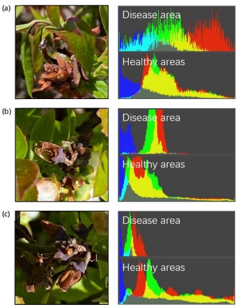
Second, the tests on different levels of shading demonstrated the effectiveness of disease extraction in HSV space, which was better and more stable than that in RGB color space, as shown in Fig. 14a-c. There existed a substantial disparity between the two extraction approaches in addressing the interference of shading on disease symptoms. Disease extraction using HSV was more stable across different levels of shading whereas disease extraction using RGB was more sensitive to light changes. A huge number of pixels in the diseased area was lost (which became empty in the diseased area) in the RGB extraction when the diseased symptom was heavily shaded. The explanation is that when the disease symptom was under normal light conditions, the most significant representation of disease visual symptom (red color), i.e., the pixel values in R channel was concentrated on the right of the histogram. However, the pixel values R channel shifted to the left when the diseased area was shaded. This shift due to illuminance change makes disease extraction using RGB color space a less applicable option compared to HSV, in which a homogenous parameter setting can be satisfied.

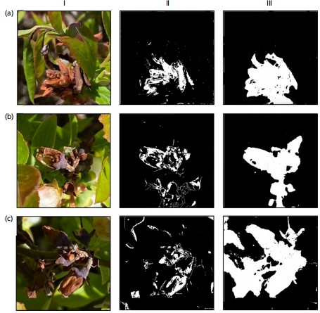
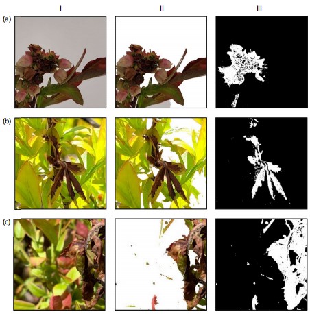
Moreover, to validate the generality of the proposed method in different scenarios with varying background complexity, three types of images were selected: No background (taken at lab view) (Fig. 15a), simple background (Fig. 15b) and complex background (Fig. 15c). In this case, the original image is shown in Fig. 15I, the de-blurred image is shown in Fig. 15b and the effects of disease extraction are displayed in Fig. 15c. The estimated severity for the lab view image was 17.4% with a relative error of 1.2%; the estimated severity for the simple background image was 8.9% with a relative error of 2.2%; the estimated severity for the complex background images was 25.2% with a relative error of 3.7%. An expanded validation on 50 images in each background type was conducted. Overall, current study method using lab view images achieved an average relative error of 1.75%, while the simple and complex backgrounds achieved 2.75 and 4.80%, respectively. Although the relative error in complex backgrounds was twice higher as that in the lab view images, less than 4% of relative error in field applications is still promising.

Fig. 12: Comparison of the deblurring effectiveness of our method with two recently developed methods on four original images

Fig. 13(a-b): Verification of disease extraction methods using HSV or RGB color space on two original images (a-b) Typical symptoms of mummy berry disease, (a) Mummy berry disease on flowers and (b) Mummy berry disease on leaves I: Original image, II: Image after deblurring, III: Disease symptom extracted using HSV color space and IV: Diseased symptom extracted using RGB color space, respectively

Fig. 14(a-c): Comparison of disease extraction effectiveness using HSV or RGB color space between different levels of shading on diseased symptoms, (a) No shading, (b) Moderate shading and (c) Severe shading I: Original image, II: Disease symptoms extracted under RGB space and III: Disease symptoms extracted under HSV space

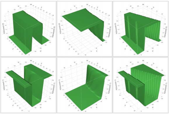
This study conducted segmentation of disease from healthy regions on the randomly selected 200 blueberry images (100 each for mummy berry disease on flowers and mummy berry disease on leaves from the original dataset). The bootstrap forest model learned the decision boundary (function) that can distinguish diseased parts from healthy areas with an accuracy of over 97% (Fig. 16) in the HSV color space based on the 5-fold cross-validation. Comparatively, the same bootstrap forest model in the RGB color space only achieved 80% accuracy, which was significantly lower and less applicable. This large gap between RGB and HSV approaches was probably due to the superior capability to deal with light variations in field scenarios. Then the learned bootstrap forest model can be used as a classifier to automatically differentiate diseased parts from healthy parts in the HSV color space.

Images acquired in field conditions are susceptible to changing light, occlusion and shadows, i.e., they are more sensitive to brightness. As a less homogeneous color space, all three components of RGB are closely related to luminance, i.e., whenever the luminance changes, all three components change accordingly. This is a big defect for RGB to deal with visual trait changes under varying light conditions. Based on the RGB color space analysis conducted on our blueberry disease images, it is clear that under normal light conditions, mummy berry disease has relatively high values in the R channel. However, the R values shift to left when the diseased area is shaded (Fig. 17). This requires different parameter settings for various light conditions, which is much less feasible in practical applications. On the contrary, the HSV space with three channels of hue, saturation and lightness can effectively deal with color changes due to varying light. Our experiments on field images showed that the extraction effect of the foci by HSV was much better than that of the RGB method. This is because, under the HSV space, it is easier to track objects of a certain color than RGB.

Fig. 15(a-c): Comparison of disease extraction effectiveness between different background complexities. (a) Disease image was taken at lab condition (no or clear background), (b) Disease image with simple background and (c) Complex background is taken from field view I: Original, II: Deblurred images and III: Extracted symptoms

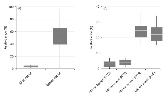
Testing accuracy of severity estimation: After the verification process, the validation process was taken on the whole mummy berry disease dataset with 400 images to statistically test its effectiveness. Deblurring is a critical step in removing irrelevant elements in a given image to accurately estimate disease severity. Figure 18a showed that the average relative error of severity estimations using the deblurring process was 3.65 with a 95% CI between 3.06 and 4.24%. However, the relative error increased to 50.29% (95% CI between 41.09 and 59.49%), which was 13 times higher when the deblurring process was not applied. This significant improvement highlighted the importance of deblurring in removing irrelevant elements and validated our assumption.

The effectiveness of disease extraction using HSV was also statistically significantly different from the approach using RGB (Fig. 18b). For the two typical symptoms, i.e., mummy berry disease on flowers and mummy berry disease on leaves, extraction under HSV achieved the average relative error of 3.07 and 4.19%, respectively. Whereas extraction under RGB had much higher relative errors, which were 24.74 and 22.34%, respectively. This result also proved that current study method can effectively and accurately estimate the severity across different types of symptoms.

Fig. 16: Decision boundaries learned by the bootstrap forest model for classification between diseased and healthy areas as a function of a nonlinear combination of the three features H, S and V in the HSV color space

This study presented a fast and accurate severity estimation algorithm for wild blueberry diseases by utilizing computer vision-based techniques. In current study method, two key innovations were established to solve two problems for analyzing field-taken images. Firstly, this study employed a novel deblurring process using defocus estimation to effectively remove blurred backgrounds so that the diseased and healthy target organs can be separated from the irrelevant background. This approach was also enhanced by using adjustable parameter settings so that low-quality images such as those without clear focus could be properly handled. Secondly, by converting RGB features into HSV space following a machine learning model bootstrap forest, diseased parts can be accurately segmented from healthy parts from the output of the first step. This approach can effectively remove the negative impact of light variations such as shading on diseased organs, which makes it an applicable and promising method in real farming conditions.

Firstly, this study effectively removes irrelevant objects from the images for severity estimation through the means of deblurring. Separating irrelevant background (such as soil, sky and other plants) from the foreground consisting of only diseased and healthy plant organs is a critical step. Many approaches using machine learning methods have been developed to deal with the blurry parts of images for disease extraction and severity estimation^44,45. Two types of cutting-edge methods have been developed recently. One is to directly decide the blur and sharp boundaries based on the sharpness of the image. The other is to achieve defocus blur separation through depth maps. Yi and Eramian⁴⁶ proposed a simple but effective clarity metric, which was based on the distribution of uniform local binary patterns (LBP) in blurred and non-blurred image regions. This method directly utilizes the sharpness of an image to measure blurry areas. However, the boundaries in the segmentation maps obtained appear jagged if there is a significant depth discontinuity between the foreground and background. This defect is because sharpness is measured locally. When using local windows, regions with different levels of sharpness are inevitably merged, especially near the edges where depth discontinuity occurs. Zhuo and Sim³⁹ used edge width as a reference for depth measurement under the assumption that edges in blurred regions are wider than those in sharp regions. The key point is that a continuous defocus map is obtained by propagating the sharpness measures at the edges to the rest of the image using image matting³⁶. Their approach utilizes the depth information of the image to distinguish clear and blurry areas but relies on high-quality images with a clear focus.

Fig. 17(a-c): RGB Histogram of pixels for diseased and healthy areas under three shading levels, (a) No shading, (b) Moderate shading and (c) Severe shading

Fig. 18(a-b): Results of disease severity estimation on the whole blueberry disease image dataset with 400 sample images, (a) Comparison of the relative error between methods with or without the process of deblur and (b) Comparison of the relative error between disease discrimination between HSV and RGB color space MB: Mummy berry disease

Secondly, this study extracts the disease areas under different lighting conditions. Previous disease extraction methods in HSV space by Hamuda et al.⁴⁷, Khan and AlGhamdi⁴⁸ and Waldamichael et al.⁴⁹, relied on high-quality images captured in controlled laboratory environments, avoiding light interferences present in field conditions. This method employed a machine learning model bootstrap forest to automatically learn classification parameters in the HSV space, achieving an accuracy of 97% based on 5-fold cross validation on 360,000-pixel samples. It enabled one parameter setting for various light conditions while keeping high disease extraction accuracy.

Finally, the method proposed in this study is compared with similar methods and the advantages of this article are analyzed. There are two major approaches for disease severity estimation in crops: Quantitative assessment based on image segmentation of diseased areas and graded qualitative assessment. Wang et al.⁵⁰ proposed a two-stage cucumber leaf disease severity classification model with the fusion of DeepLabV3+ and U-Net (DUNet) in complex backgrounds. They calculated the severity of the disease by calculating the ratio of the area of the disease spot to the total area and the average accuracy rate reached 92.85%. Guo et al.⁵¹ segmented the stripe rust spots of wheat spectral images and graded the disease level by calculating the spot area to the total leaf area, with an accuracy of 98.15%. These studies used traditional image processing methods on images with simple and clear backgrounds in controlled environments. One obvious disadvantage of these methods is that without extraction of depth information, they are not able to deal with images with complex backgrounds and differentiate diseased objects. However, applications in real farming conditions often encounter images with occlusions and interferences. The study approach uses a novel deblurring technique to effectively remove irrelevant backgrounds by considering the depth of information of relevant objects. Furthermore, with the assistance of parameter adjustments, this approach can also effectively extract diseased objects from low-quality images, showing robustness in field applications.

Deep learning methods in disease severity estimation are important for efficient disease management^52,53. Since training deep neural networks requires a large number of labeled images, measuring and rating severity for these images are very labor intensive. Therefore, they have been widely used to classify the level of disease severity, instead of giving an accurate rating percentage. In this framework, the disease severity is manually divided into several classes by experts, from which the convolutional neural networks can be trained⁵⁴. Then the level of severity in the input images can be directly classified with powerful automatic feature learning capabilities, avoiding image segmentation. Although a direct comparison between our method and deep learning approaches has not been done, this study can still assess the potential role of our method from another perspective. Having the capability of accurately rating disease severity in field images, our method can serve as an effective auto-labeling tool to assist in labeling or grading the severity of diseases in a given image with blueberry disease. By doing so, the number of labeled images can be sufficiently increased, which will expand the number of samples which deep learning methods can be applied. This work therefore provides a solid foundation for deep learning-based approaches to disease severity estimation by solving the labor-intensive rating problem.

CONCLUSION

To conclude, we developed a fast and accurate severity estimation algorithm for wild blueberry diseases by utilizing computer vision-based techniques. Based on the statistical analysis from a large amount of field-collected images, our method can effectively identify diseased and healthy plant organs as foreground in an image and make an accurate estimation with less than average 5% relative error. There are two innovations in our approachin. First, we employed a novel deblurring process using defocus estimation to effectively remove blurred backgrounds so that the diseased and healthy target organs can be separated from the irrelevant background. This method was also enhanced by using adjustable parameter settings so that low-quality images can be properly handled. Second, by converting RGB features into HSV space following a machine learning model bootstrap forest, diseased parts can be accurately segmented from healthy parts from the output of the first step. Our method can alleviate negative impact of light variations in real farming conditions. Additionally, this approach can serve as an auto-labeling tool for the automatic rating of disease severity for field-taken images, on which deep learning models can be trained without the limitation of data scarcity.

SIGNIFICANCE STATEMENT

Blueberries, as an important economic crop worldwide, are increasingly facing significant disease issues. The purpose of this study is to estimate the severity of two common blueberry diseases using machine vision technology. The results indicate that the method proposed in this study has high accuracy and can effectively estimate the severity of blueberry diseases, which is of great significance for the prevention and treatment of blueberry diseases and precise medication.

ACKNOWLEDGMENTS

We would like to thank Drs. Seanna Annis and Frank Drummond and their graduate students for helping with the data collection.

REFERENCES

1. Yarborough, D., F. Drummond, S. Annis and J. D’Appollonio, 2017. Maine wild blueberry systems analysis. Acta Hortic., 1180: 151-160.
2. Strik, B.C. and D. Yarborough, 2005. Blueberry production trends in North America, 1992 to 2003, and predictions for growth. HortTechnology, 15: 391-398.
3. Lambert, D.H., 1990. Effects of pruning method on the incidence of mummy berry and other lowbush blueberry diseases. Plant Dis., 74: 199-201.
4. Obsie, E.Y., H. Qu and F. Drummond, 2020. Wild blueberry yield prediction using a combination of computer simulation and machine learning algorithms. Comput. Electron. Agric., 178.
5. Qu, H. and F. Drummond, 2018. Simulation-based modeling of wild blueberry pollination. Comput. Electron. Agric., 144: 94-101.
6. Mundt, C.C., 2009. The study of plant disease epidemics. HortScience, 44: 2065b-2065.
7. Shi, T., Y. Liu, X. Zheng, K. Hu, H. Huang, H. Liu and H. Huang, 2023. Recent advances in plant disease severity assessment using convolutional neural networks. Sci. Rep., 13.
8. James, W.C., 1974. Assessment of plant diseases and losses. Annu. Rev. Phytopathol., 12: 27-48.
9. Haider, W., Aqeel-Ur Rehman, N.M. Durrani and Sadiq Ur Rehman, 2021. A generic approach for wheat disease classification and verification using expert opinion for knowledge-based decisions. IEEE Access, 9: 31104-31129.
10. Neupane, K. and F. Baysal-Gurel, 2021. Automatic identification and monitoring of plant diseases using unmanned aerial vehicles: A review. Remote Sens., 13.
11. Qu, H. and M. Sun, 2022. A lightweight network for mummy berry disease recognition. Smart Agric. Technol., 2.
12. Obsie, E.Y., H. Qu, Y.J. Zhang, S. Annis and F. Drummond, 2023. Yolov5s-CA: An improved Yolov5 based on the attention mechanism for mummy berry disease detection. Agriculture, 13.
13. Karlekar, A. and A. Seal, 2020. SoyNet: Soybean leaf diseases classification. Comput. Electron. Agric., 172.
14. Lin, H.Y., C.C. Chang and X.H. Chou, 2017. No-reference objective image quality assessment using defocus blur estimation. J. Chin. Inst. Eng., 40: 341-346.
15. Tian, Y., H. Duan, R. Luo, Y. Zhang and W. Jia et al., 2019. Fast recognition and location of target fruit based on depth information. IEEE Access, 7: 170553-170563.
16. Zhuang, Z., T. Li, H. Wang and J. Sun, 2024. Blind image deblurring with unknown kernel size and substantial noise. Int. J. Comput. Vis., 132: 319-348.
17. Zhang, K., W. Ren, W. Luo, W.S. Lai, B. Stenger, M.H. Yang and H. Li, 2022. Deep image deblurring: A survey. Int. J. Comput. Vis., 130: 2103-2130.
18. Ma, H., S. Liu, Q. Liao, J. Zhang and J.H. Xue, 2022. Defocus image deblurring network with defocus map estimation as auxiliary task. IEEE Trans. Image Process., 31: 216-226.
19. Guo, Q., W. Feng, R. Gao, Y. Liu and S. Wang, 2021. Exploring the effects of blur and deblurring to visual object tracking. IEEE Trans. Image Process., 30: 1812-1824.
20. Barbedo, J.G.A., 2016. Expert systems applied to plant disease diagnosis: Survey and critical view. IEEE Lat. Am. Trans., 14: 1910-1922.
21. Arsenovic, M., M. Karanovic, S. Sladojevic, A. Anderla and D. Stefanovic, 2019. Solving current limitations of deep learning based approaches for plant disease detection. Symmetry, 11.
22. Pallathadka, H., P. Ravipati, G.S. Sajja, K. Phasinam, T. Kassanuk, D.T. Sanchez and P. Prabhu, 2022. Application of machine learning techniques in rice leaf disease detection. Mater. Today: Proc., 51: 2277-2280.
23. Trivedi, V.K., P.K. Shukla and A. Pandey, 2022. Automatic segmentation of plant leaves disease using min-max hue histogram and k-mean clustering. Multimed. Tools Appl., 81: 20201-20228.
24. Patil, M.A. and M. Manohar, 2022. Enhanced radial basis function neural network for tomato plant disease leaf image segmentation. Ecol. Inf., 70.
25. Barbedo, J.G.A., 2016. A review on the main challenges in automatic plant disease identification based on visible range images. Biosyst. Eng., 144: 52-60.
26. Florence, J. and J. Pscheidt, 2017. Monilinia vaccinii-corymbosi apothecial development associated with mulch depth and timing of application. Plant Dis., 101: 807-814.
27. Harteveld, D.O.C. and T.L. Peever, 2018. Timing of susceptibility of highbush blueberry cultivars in Northwestern Washington to Monilinia vaccinii‐corymbosi, the cause of mummy berry. Plant Pathol., 67: 477-487.
28. Yang, J., Y. Liu, Q. Meng and R. Chu, 2015. Objective evaluation criteria for stereo camera shooting quality under different shooting parameters and shooting distances. IEEE Sensors J., 15: 4508-4521.
29. Nalwa, V.S. and T.O. Binford, 1986. On detecting edges. IEEE Trans. Pattern Anal. Mach. Intell., PAMI-8: 699-714.
30. Zhang, X., R. Wang, X. Jiang, W. Wang and W. Gao, 2016. Spatially variant defocus blur map estimation and deblurring from a single image. J. Visual Commun. Image Represent., 35: 257-264.
31. Hummel, R.A., B. Kimia and S.W. Zucker, 1987. Deblurring gaussian blur. Comput. Vision Graphics Image Process., 38: 66-80.
32. Lim, C.L., R. Paramesran, W.A. Jassim, Y.P. Yu and K.N. Ngan, 2016. Blind image quality assessment for Gaussian blur images using exact Zernike moments and gradient magnitude. J. Franklin Inst., 353: 4715-4733.
33. Canny, J., 1986. A computational approach to edge detection. IEEE Trans. Pattern Anal. Mach. Intell., 8: 679-698.
34. Al-Nasrawi, M., G. Deng and B. Thai, 2018. Edge-aware smoothing through adaptive interpolation. Signal Image Video Process., 12: 347-354.
35. Wang, Z., X. Ye, B. Sun, J. Yang, R. Xu and H. Li, 2020. Depth upsampling based on deep edge-aware learning. Pattern Recognit., 103.
36. Levin, A., D. Lischinski and Y. Weiss, 2008. A closed-form solution to natural image matting. IEEE Trans. Pattern Anal. Mach. Intell., 30: 228-242.
37. Yuan, F., Y. Zhou, X. Xia, J. Shi, Y. Fang and X. Qian, 2020. Image dehazing based on a transmission fusion strategy by automatic image matting. Comput. Vision Image Understanding, 194.
38. Liu, X., H. Zhang, Y.M. Cheung, X. You and Y.Y. Tang, 2017. Efficient single image dehazing and denoising: An efficient multi-scale correlated wavelet approach. Comput. Vision Image Understanding, 162: 23-33.
39. Zhuo, S. and T. Sim, 2011. Defocus map estimation from a single image. Pattern Recognit., 44: 1852-1858.
40. Datta, J. and J.K. Ghosh, 2014. Bootstrap-An exploration. Stat. Methodol., 20: 63-72.
41. Xanthopoulos, P., P.M. Pardalos and T.B. Trafalis, 2013. Linear Discriminant Analysis. In: Robust Data Mining, Xanthopoulos, P., P.M. Pardalos and T.B. Trafalis (Eds.), Springer, New York, ISBN: 978-1-4419-9878-1, pp: 27-33.
42. Fushiki, T., 2011. Estimation of prediction error by using K-fold cross-validation. Stat. Comput., 21: 137-146.
43. Park, J.S., M.S. Chung, S.B. Hwang, Y.S. Lee and D.H. Har, 2005. Technical report on semiautomatic segmentation using the adobe photoshop. J. Digital Imaging, 18: 333-343.
44. Pan, J., W. Ren, Z. Hu and M.H. Yang, 2019. Learning to deblur images with exemplars. IEEE Trans. Pattern Anal. Mach. Intell., 41: 1412-1425.
45. Huihui, Y., L. Daoliang and C. Yingyi, 2023. A state-of-the-art review of image motion deblurring techniques in precision agriculture. Heliyon, 9.
46. Yi, X. and M. Eramian, 2016. LBP-Based segmentation of defocus blur. IEEE Trans. Image Process., 25: 1626-1638.
47. Hamuda, E., B.M. Ginley, M. Glavin and E. Jones, 2017. Automatic crop detection under field conditions using the HSV colour space and morphological operations. Comput. Electron. Agric., 133: 97-107.
48. Khan, M.A. and M.A. AlGhamdi, 2024. An intelligent and fast system for detection of grape diseases in RGB, grayscale, YCbCr, HSV and L*a*b* color spaces. Multimed. Tools Appl., 83: 50381-50399.
49. Waldamichael, F.G., T.G. Debelee and Y.M. Ayano, 2022. Coffee disease detection using a robust HSV color-based segmentation and transfer learning for use on smartphones. Int. J. Intell. Syst., 37: 4967-4993.
50. Wang, C., P. Du, H. Wu, J. Li, C. Zhao and H. Zhu, 2021. A cucumber leaf disease severity classification method based on the fusion of DeepLabV3+ and U-Net. Comput. Electron. Agric., 189.
51. Guo, A., W. Huang, Y. Dong, H. Ye and H. Ma et al., 2021. Wheat yellow rust detection using UAV-based hyperspectral technology. Remote Sens., 13.
52. Wang, G., Y. Sun and J. Wang, 2017. Automatic image-based plant disease severity estimation using deep learning. Comput. Intell. Neurosci., 2017.
53. Liang, Q., S. Xiang, Y. Hu, G. Coppola, D. Zhang and W. Sun, 2019. PD²SE-Net: Computer-assisted plant disease diagnosis and severity estimation network. Comput. Electron. Agric., 157: 518-529.
54. Hayit, T., H. Erbay, F. Varçın, F. Hayit and N. Akci, 2021. Determination of the severity level of yellow rust disease in wheat by using convolutional neural networks. J. Plant Pathol., 103: 923-934.